Insert Slicer In MS Excel

This blog post demonstrates inserting a slicer, connecting a slicer to multiple PivotTables, formatting slicers for clear display, and using slicer settings to control selection behavior. 

The tutorial solves common problems that slow data analysis: it removes repetitive manual filtering, makes multi-table filtering consistent, and reduces errors from hidden or complex filter menus. 

Learn how slicers speed up dashboard interaction, make reports more intuitive for non-technical users, and provide an easy way to highlight trends and segments during presentations. 

Practical tips on sizing, alignment, and visual styling ensure slicers integrate seamlessly into professional dashboards. Let's start.

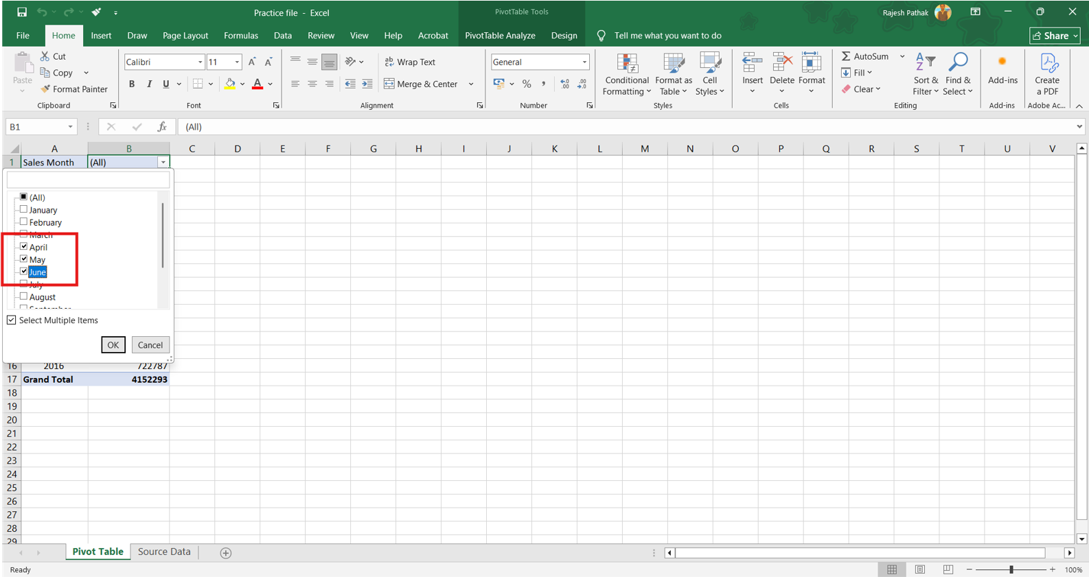
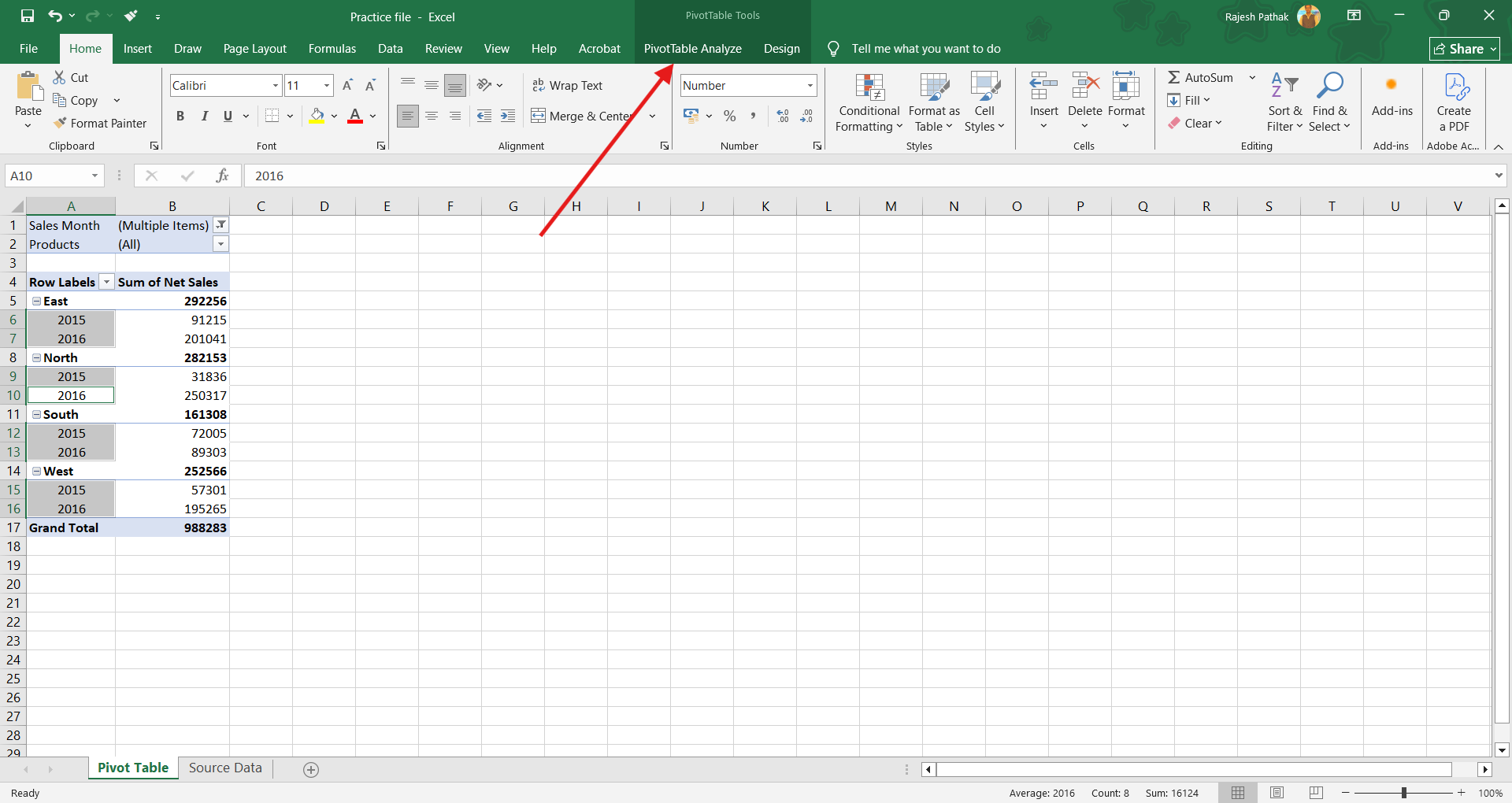
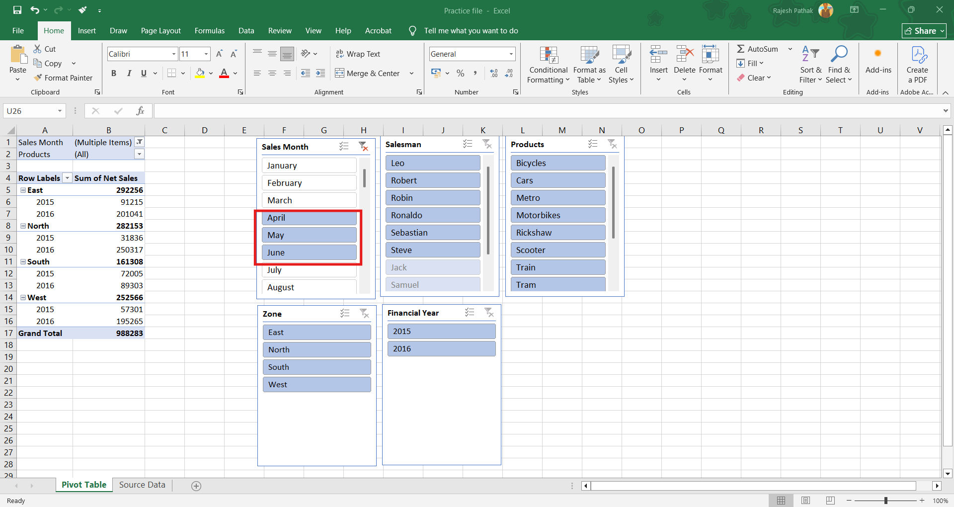
In this pivot table we have 'sales month' and 'products' in the report filter field.

When we open the filter of months, we can see that April to June months have been filtered.

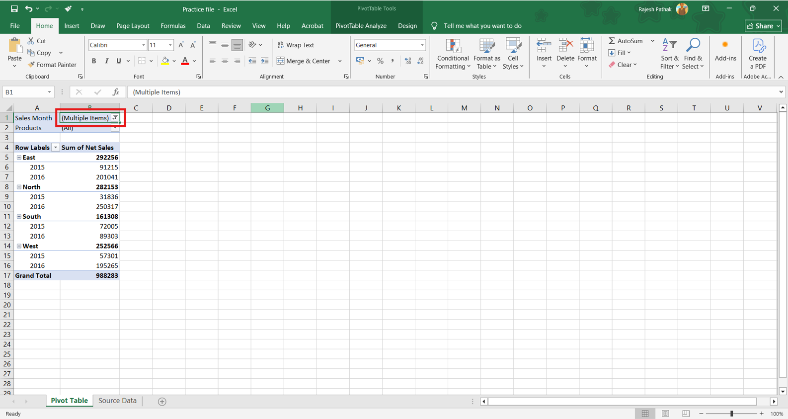
But when we come out of filter, we don't know which items have been filtered.

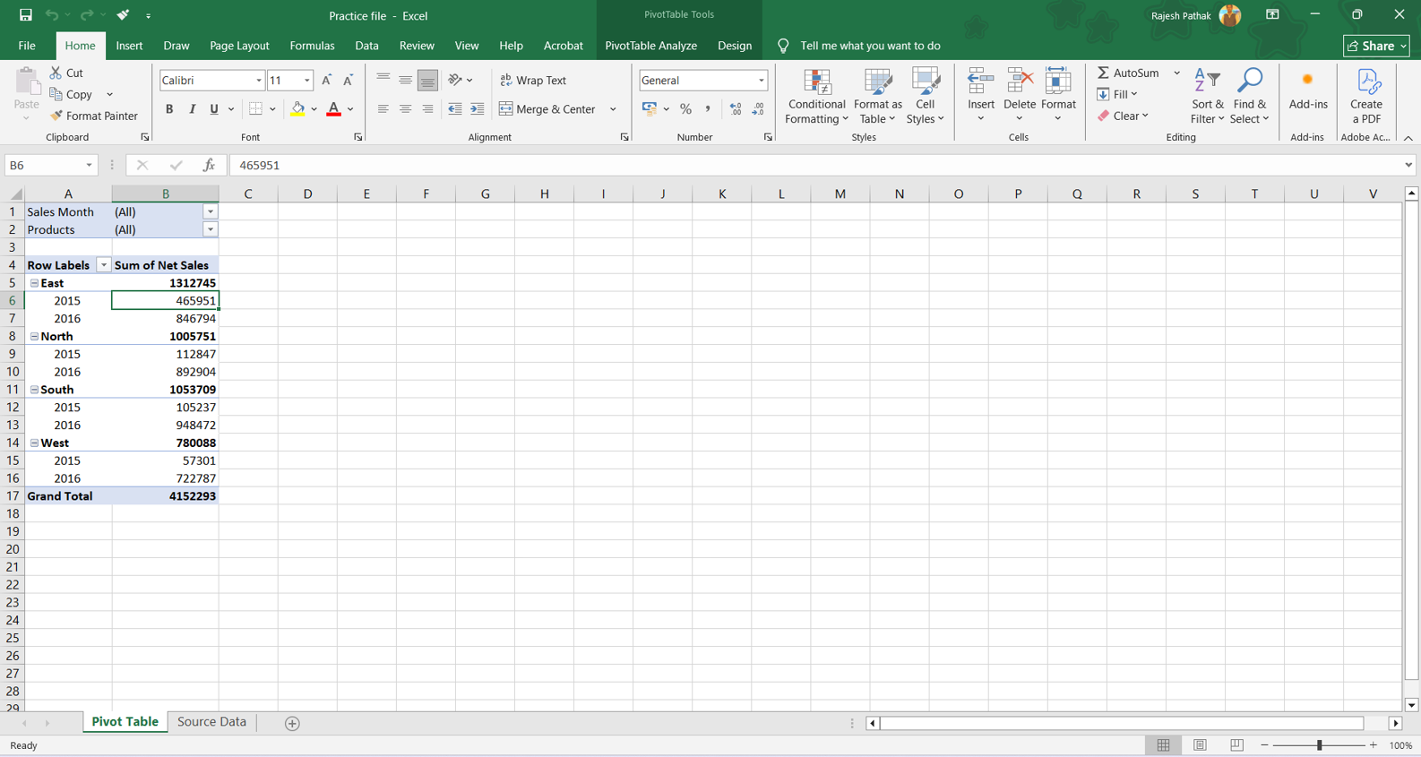
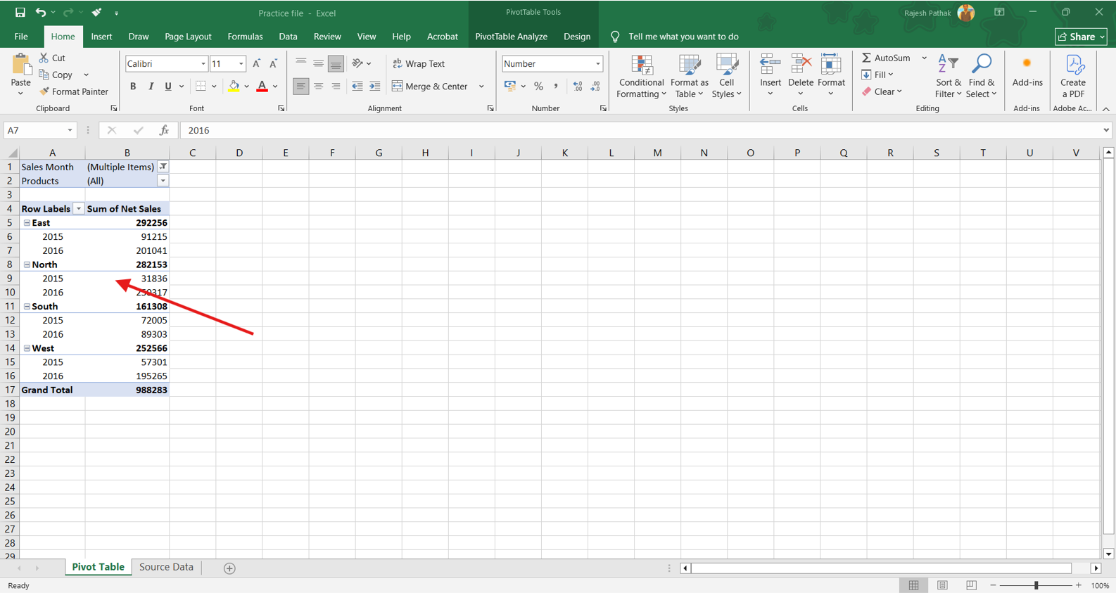
Only thing visible is 'multiple items'. This can be irritating at the time of working with data as we need to open filters each time to know which items have been filtered in the data.

This problem was solved in excel 2010 version by introducing slicers feature. Slicers are visual filter buttons which enable us to quickly filter data in an interactive way.

It also keeps both filtered and non-filtered items visible for us.

To insert slicers, place the cursor Inside pivot table.

Go to 'PivotTable Analyze' ribbon tab.

In the 'Filter' group, click on 'insert slicer' button.

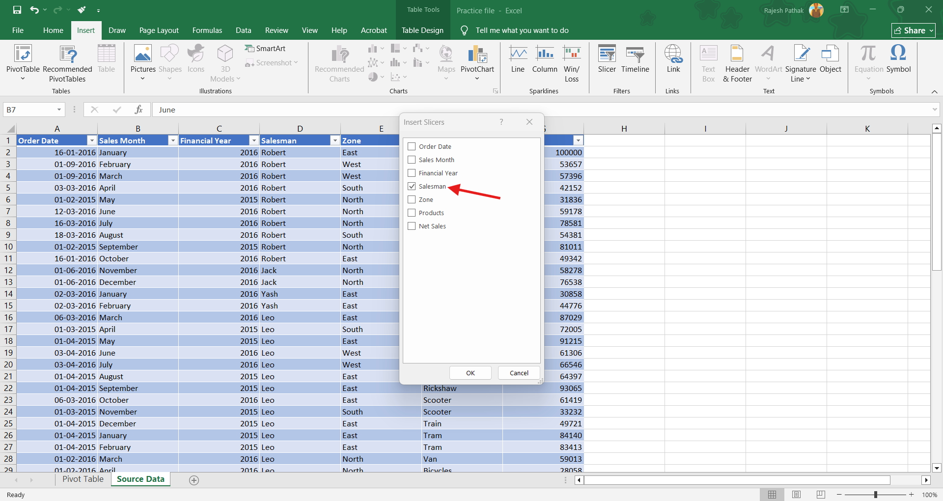
'Insert slicers' dialog box opens'. This dialog box contains all the pivot table field list items. 

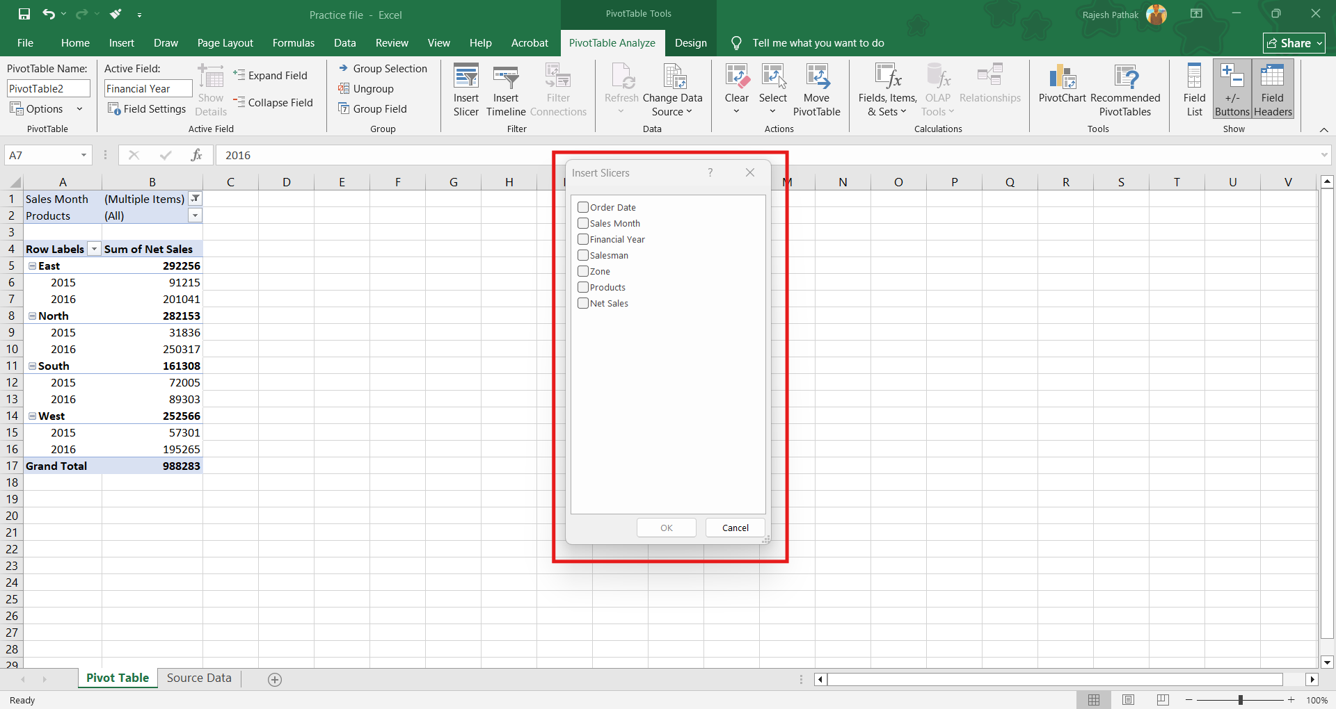
Let's insert five different slicers by selecting 'sales month', 'financial year', 'salesman', 'zone', and 'products'.

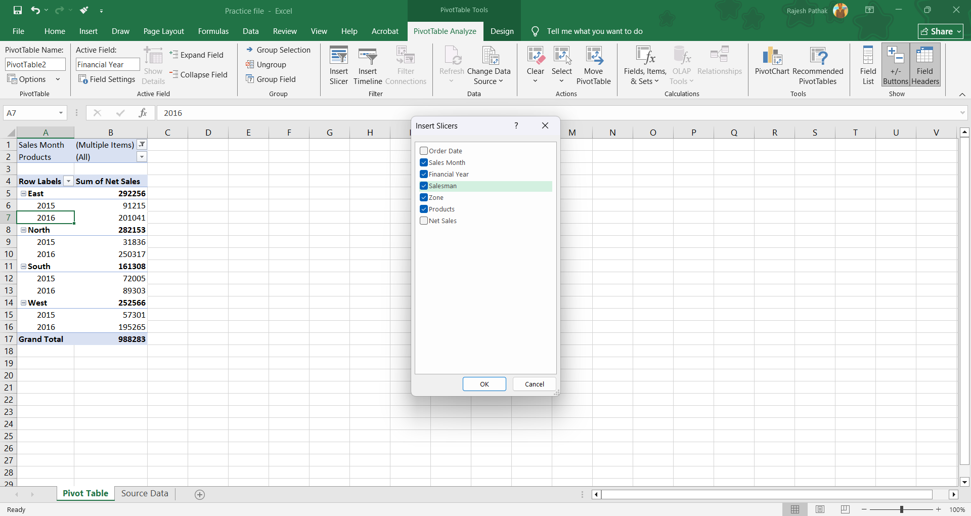
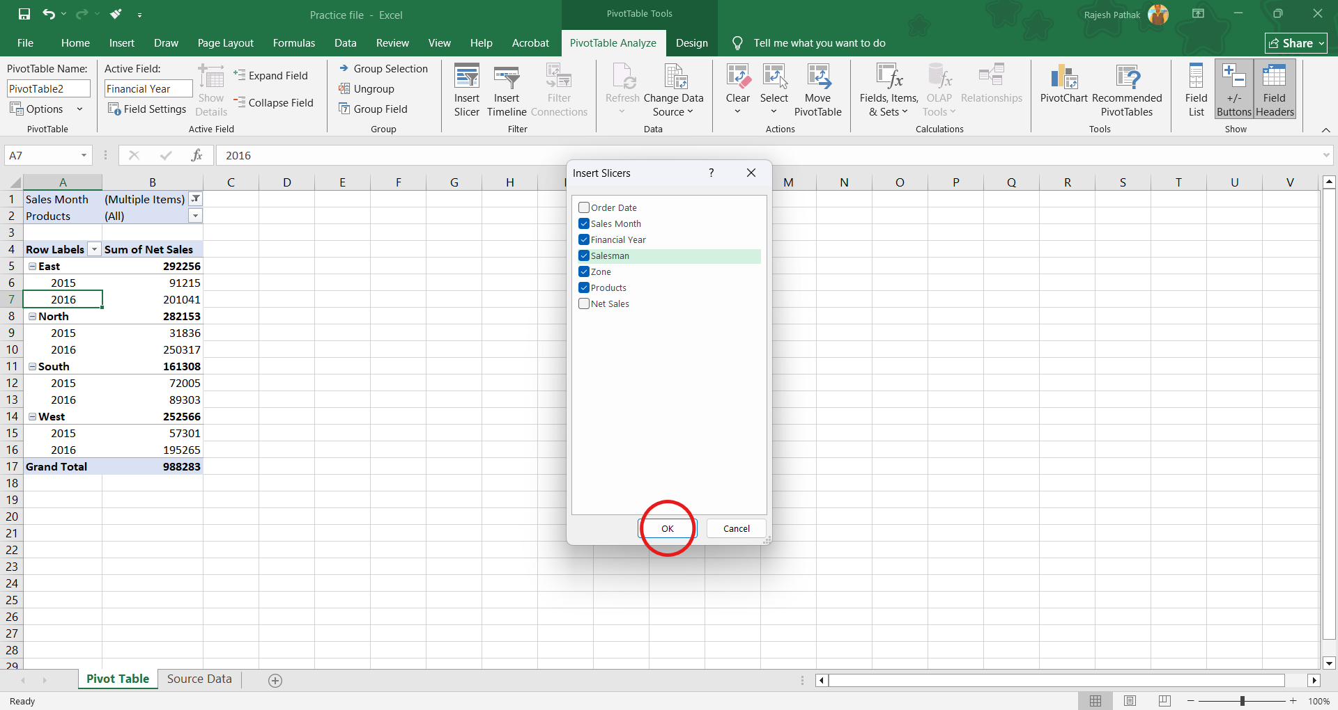
Press OK button.

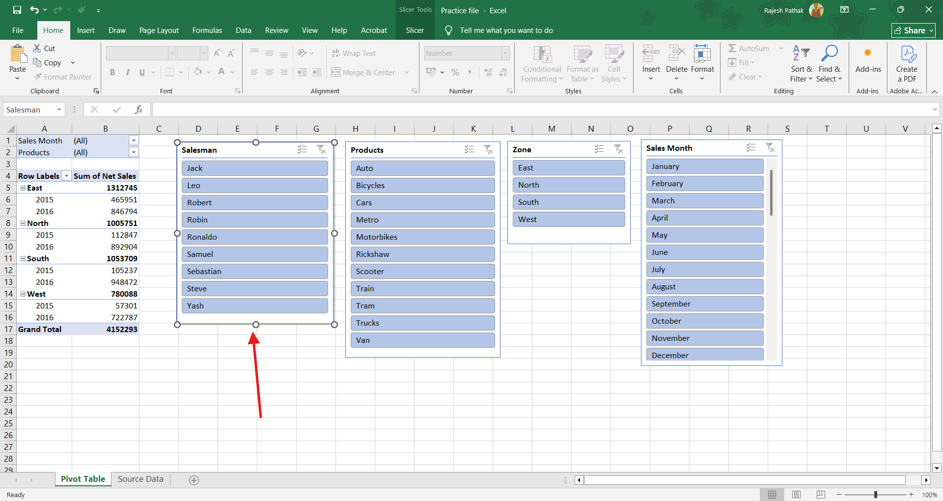
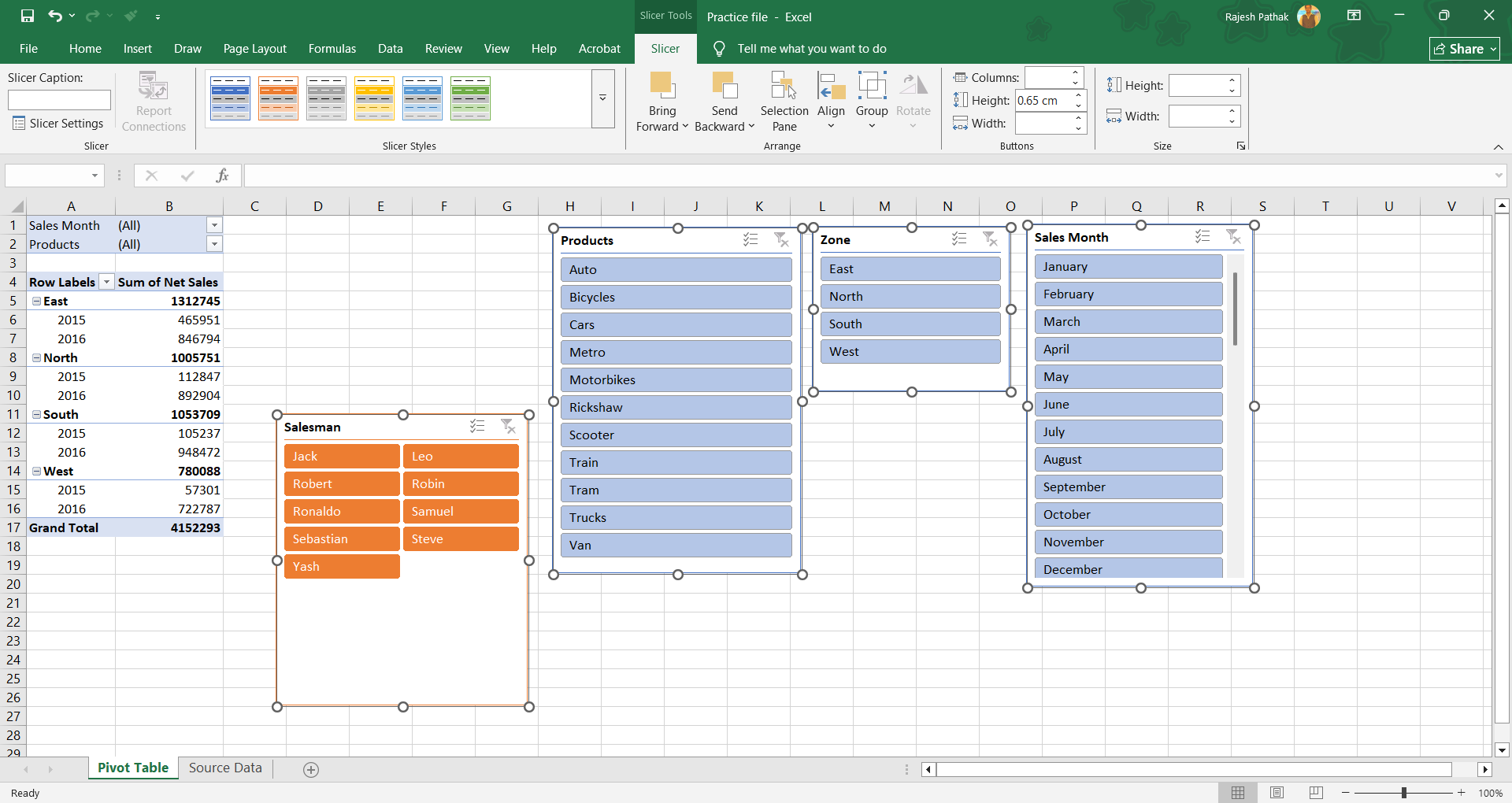
Arrange the slicers nicely in the worksheet.

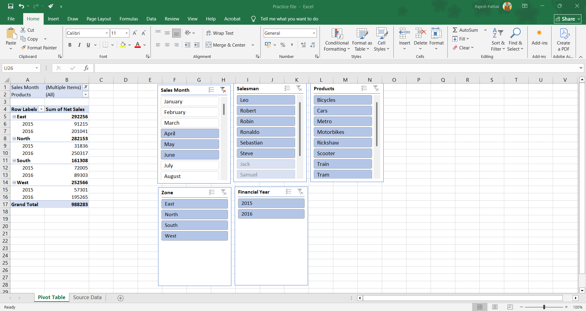
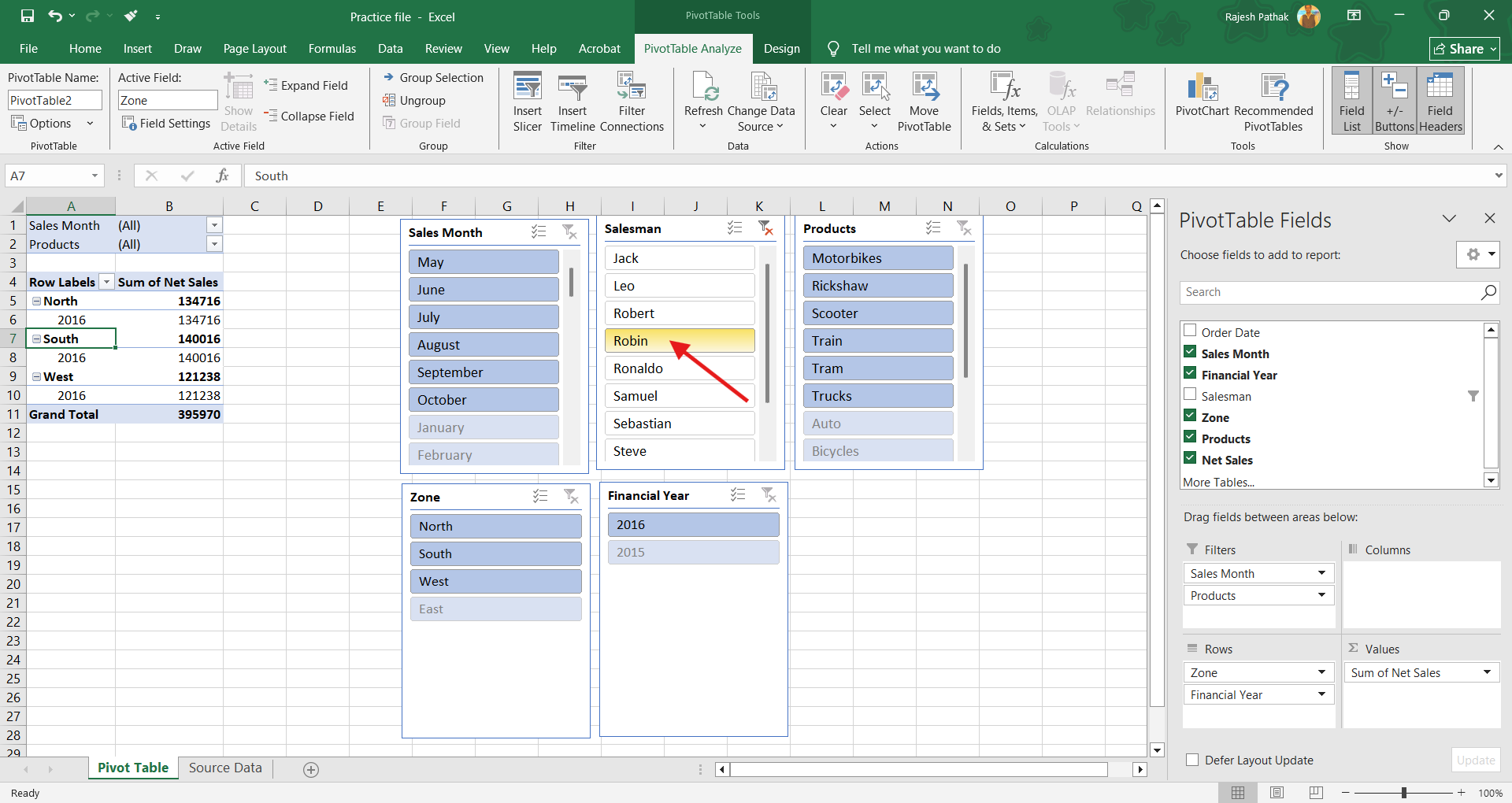
Sales months that have been filtered in the report filter area can be seen highlighted in the 'sales month' slicer.

We don't have to use report filter any more for filtering purpose. We can use these slicers to filter our data. Filtered items are highlighted in blue. Those which are not highlightedare not filtered.

To clear the filter from 'sales month' slicer, click on the top right hand corner.

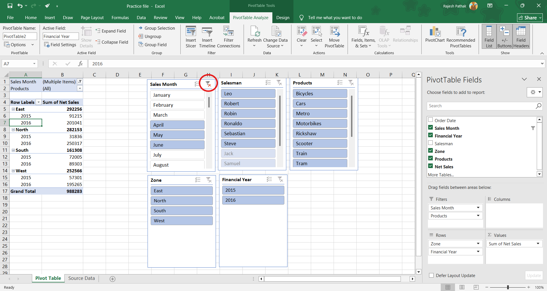
Filters are removed from slicers and report filter area.

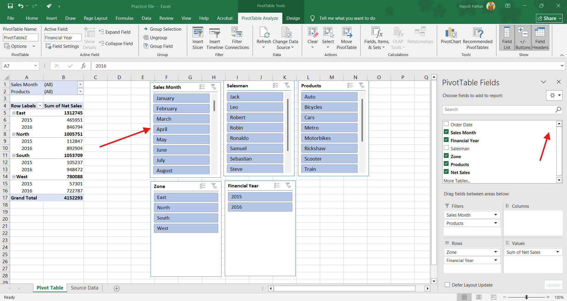
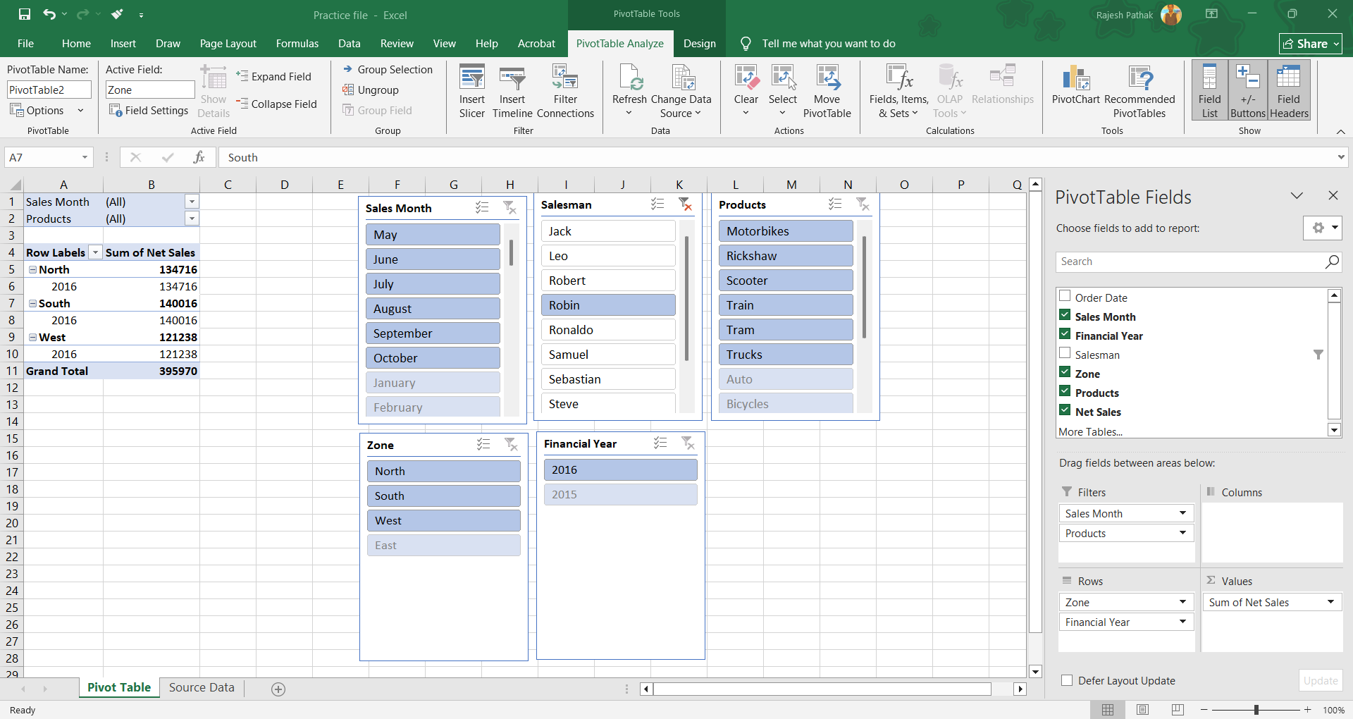
Let's click on one of the salesman's name.

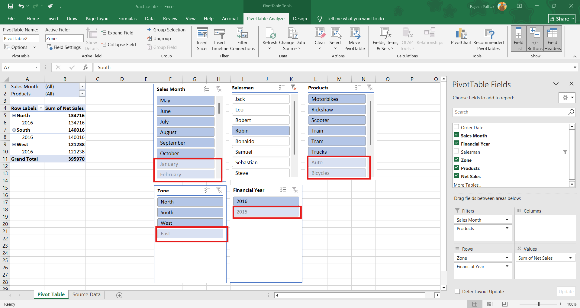
All the slicers have highlighted only the relevant sections of the filters where there are values.

Greyed items don't have values for the selected salesman. 

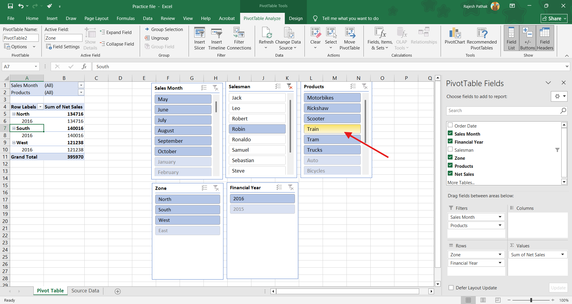
While holding control key, we can select multiple items randomly or in a row. We can select multiple items in a row together by first clicking on the first item.....then hold the shift key, and then select the last item in the row.

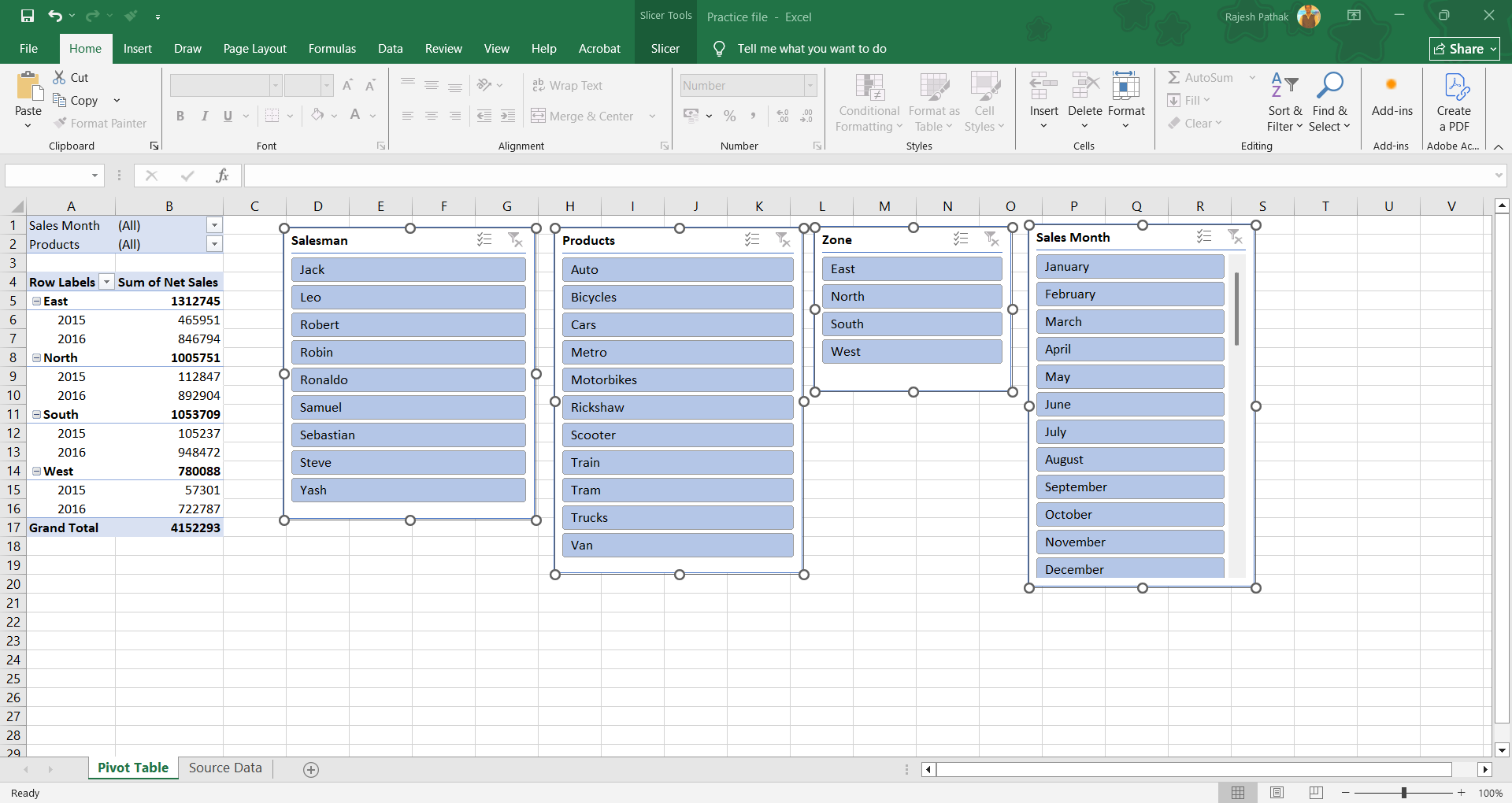
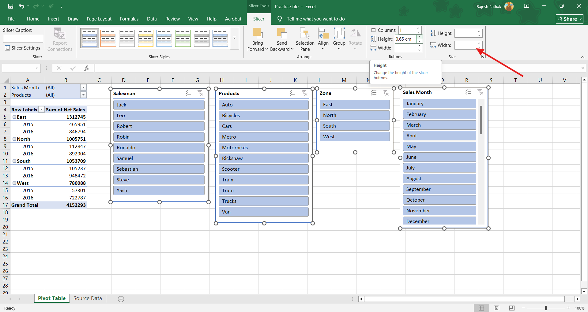
We can make changes to the size of slicer and its button. Select a slicer.

Press Control A to select all the slicers.

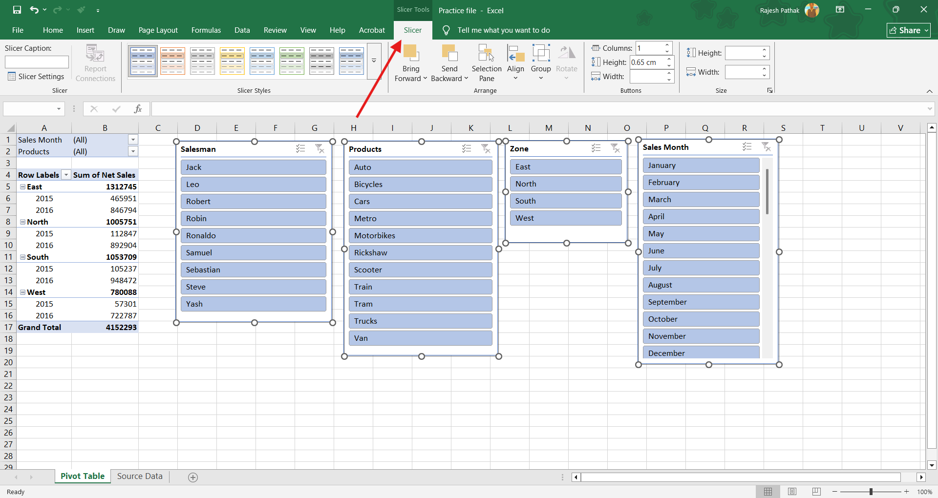
Go to 'Slicer' ribbon tab.

We can increase or decrease the height of slicer buttons.

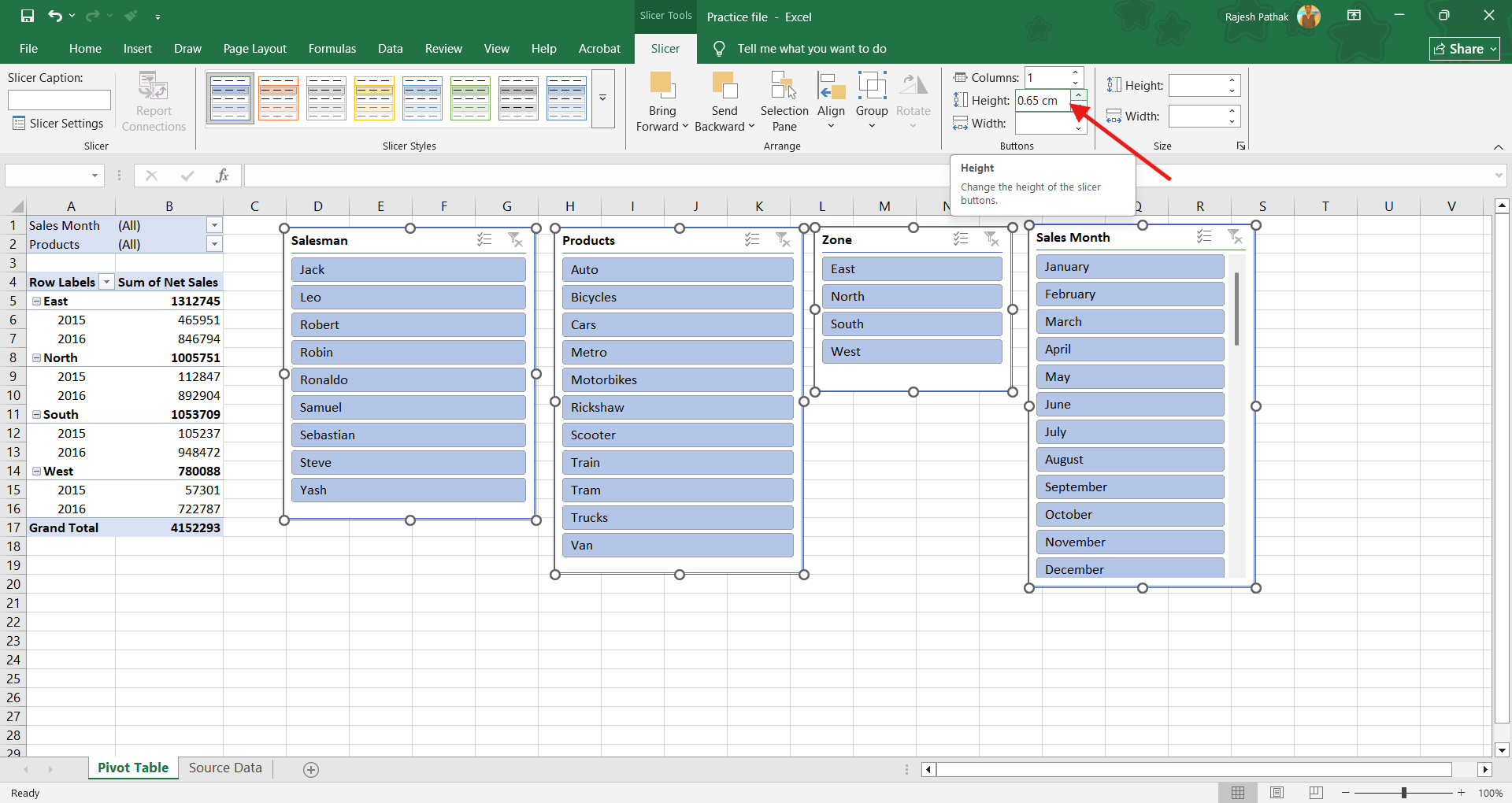
Similarly, we can increase or decrease the height of slicers.

We can also increase or decrease the width of slicers.

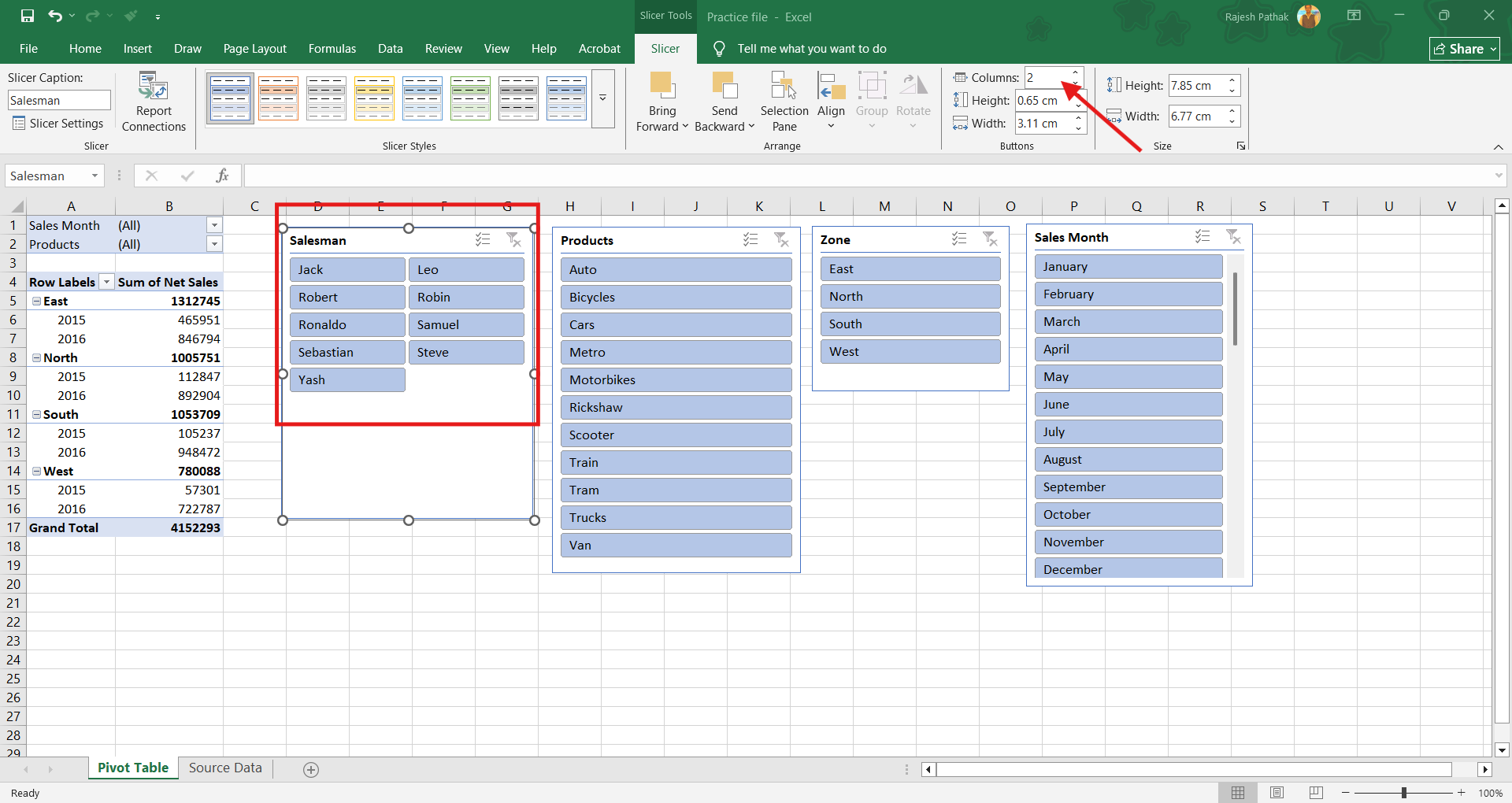
We can create more than one column to make the slicer look more elegant. Columns can be increased or decreased from 'columns' section in options tab.

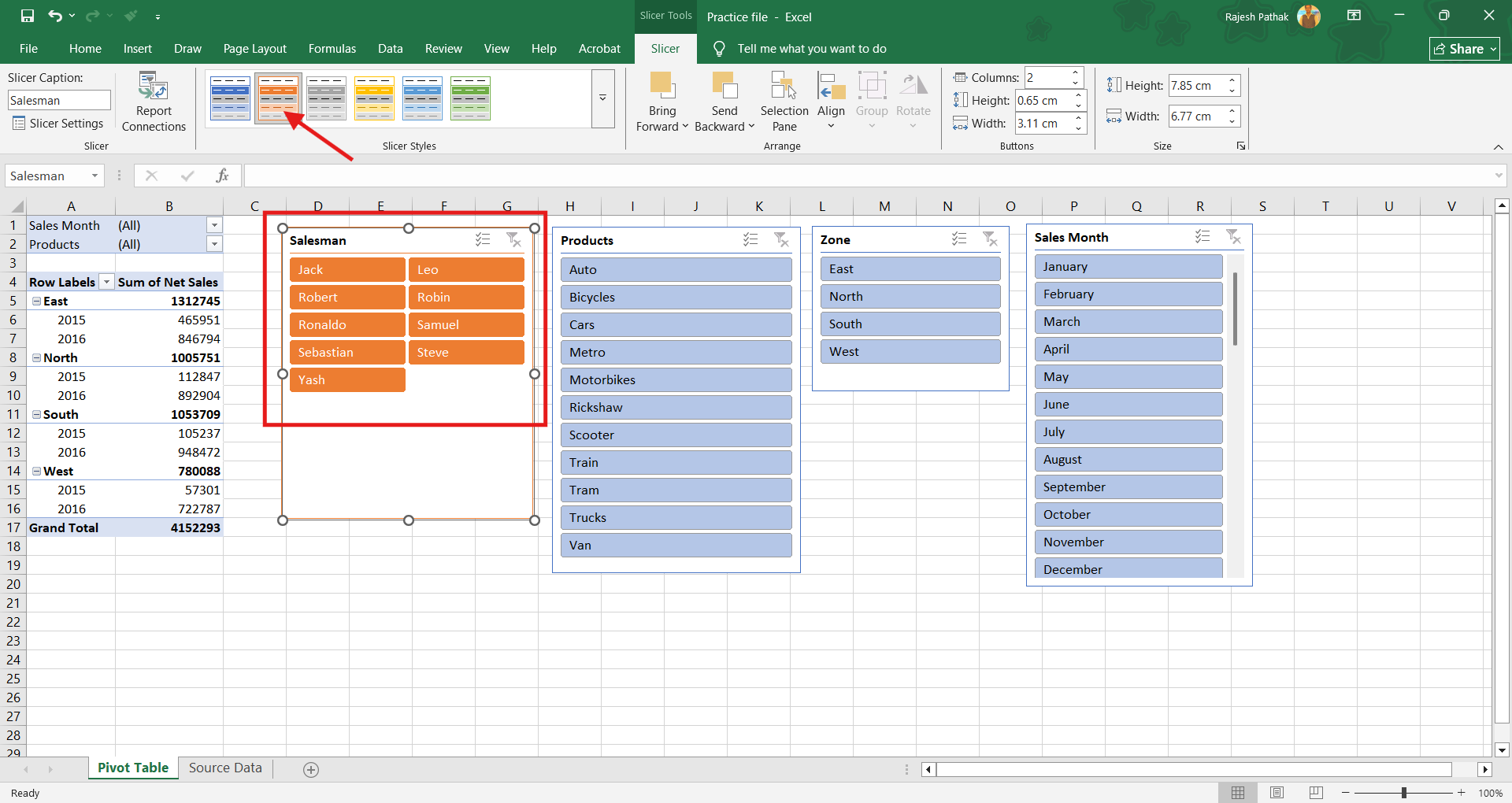
From slicer ribbon tab, we can apply different colours to different slicers to differentiate them from each other.

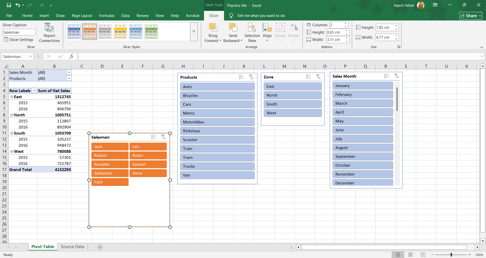
Drag one slicer to thc bottom. Now slicer arrangement is totally disturbed. But we can arrange the slicers very quickly.

Press Control A to select all slicers.

In slicer tab, click on align drop-down arrow.

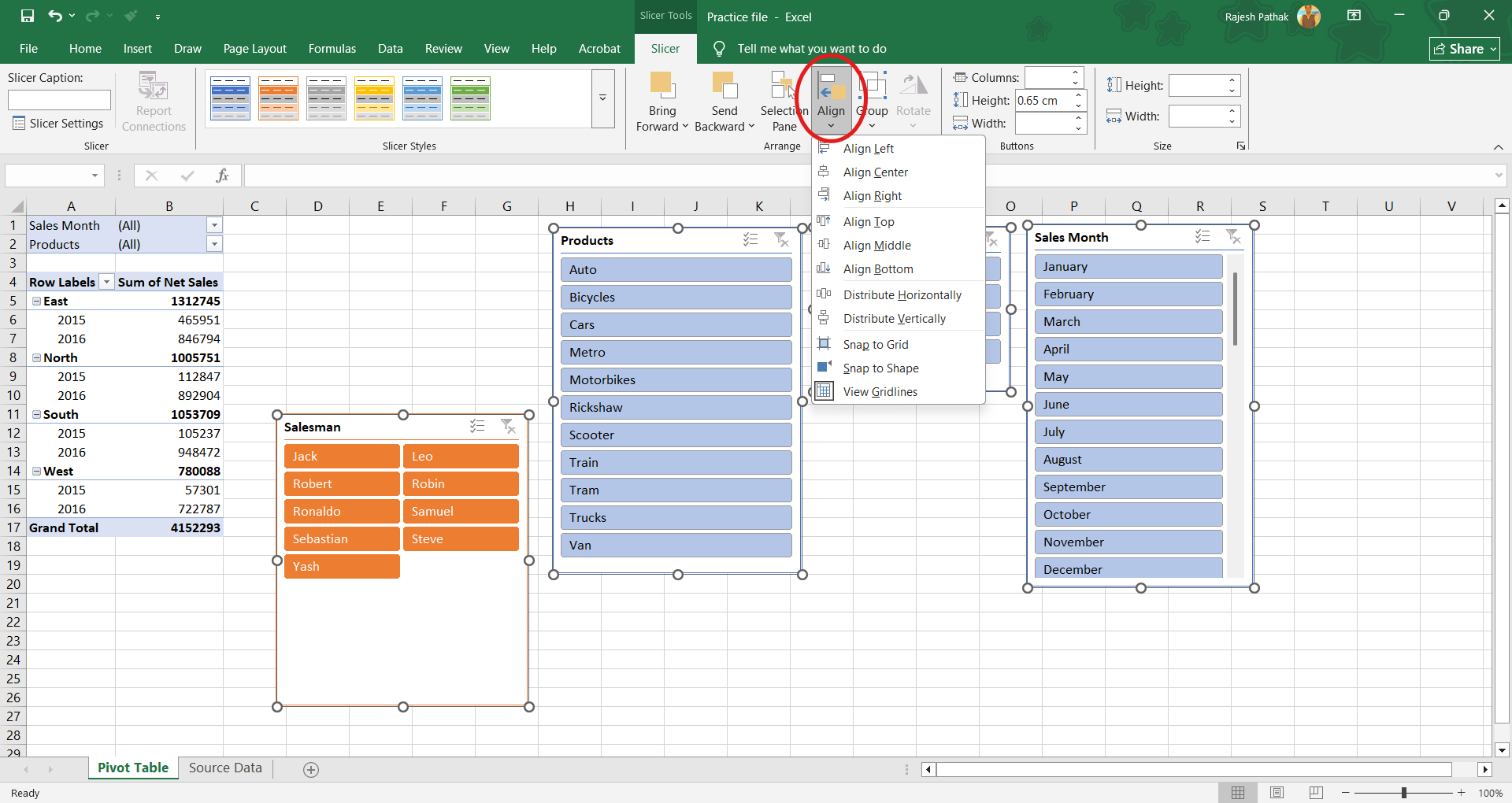
Click on align top.

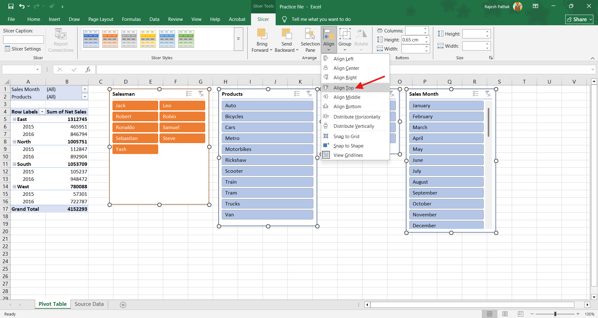
All slicers are now nicely arranged.

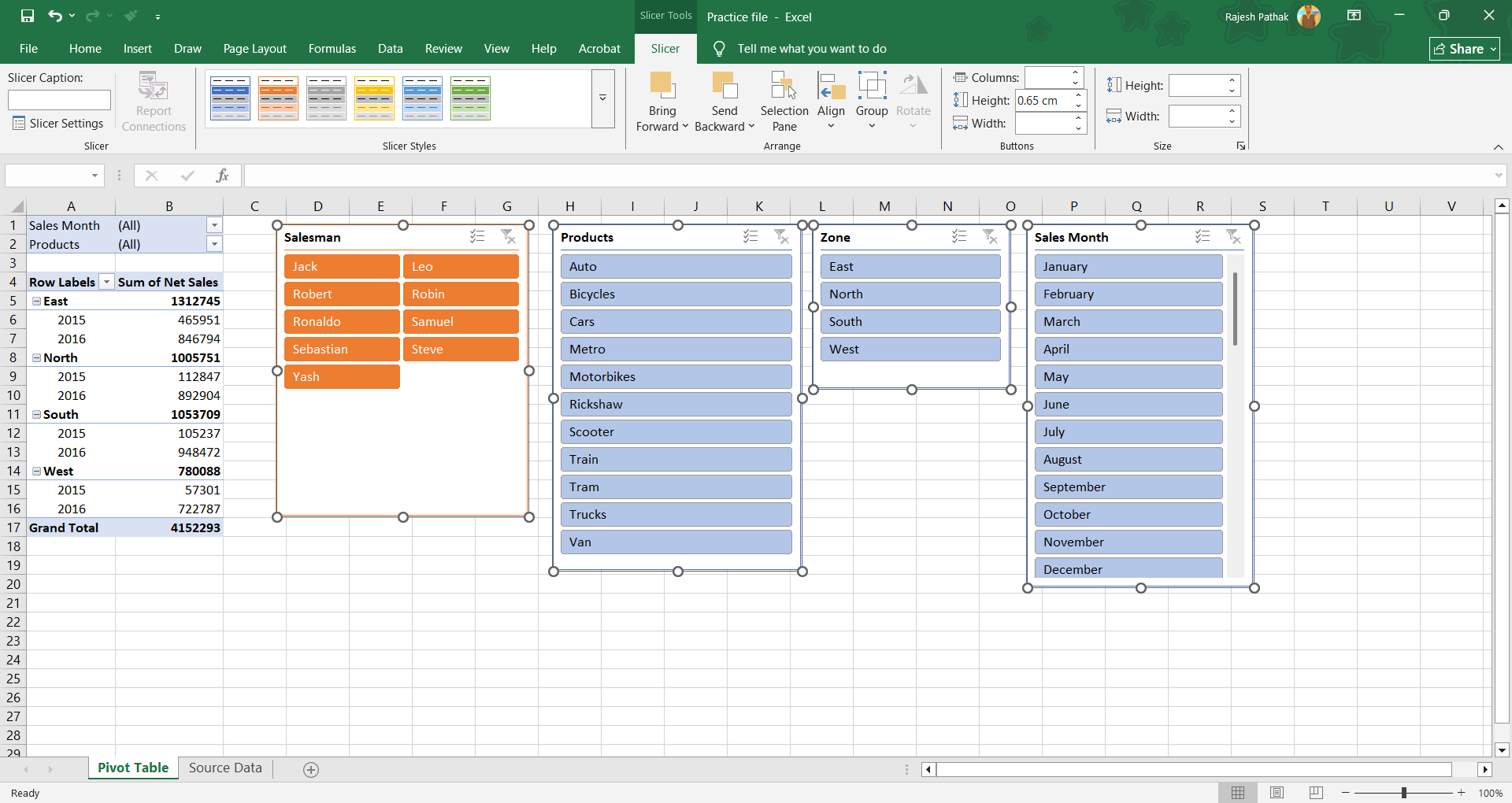
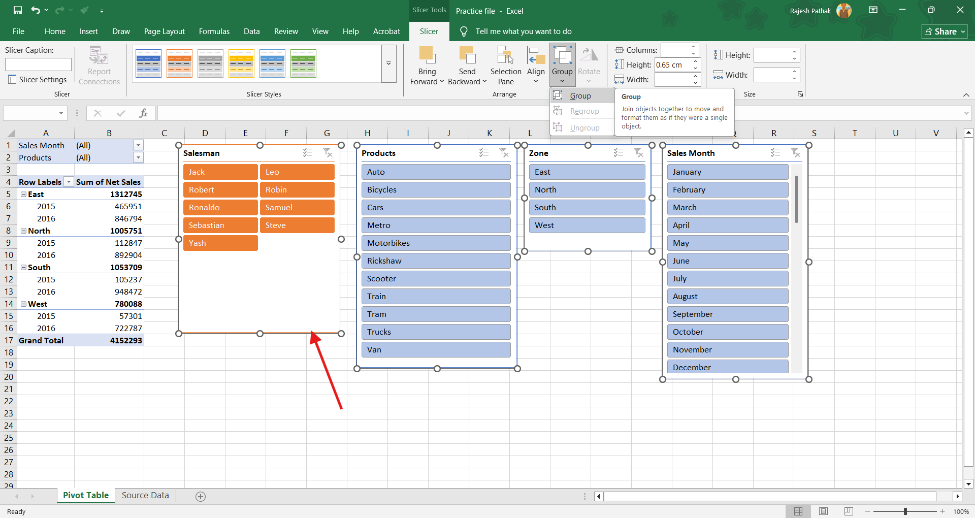
We can also group all these selected slicers. Grouping helps them to move together in the workshcct without disturbing the alignment. Keep all the slicers selected. In slicer tab, click on group drop-down arrow.

Use the outer border to move all slicers together.

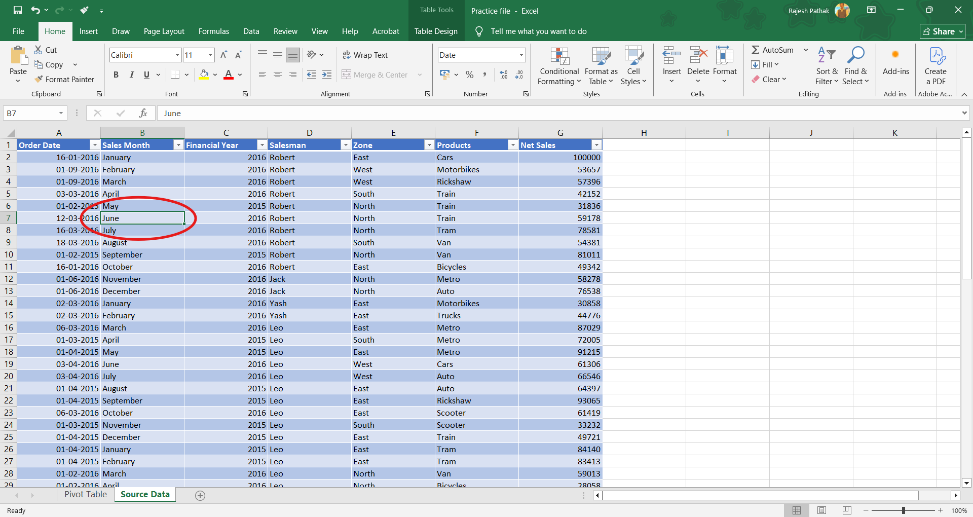
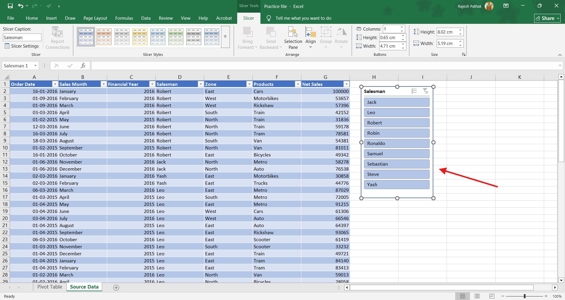
Apart from pivot tables, slicers can be used in excel tables as well. Click inside excel table.

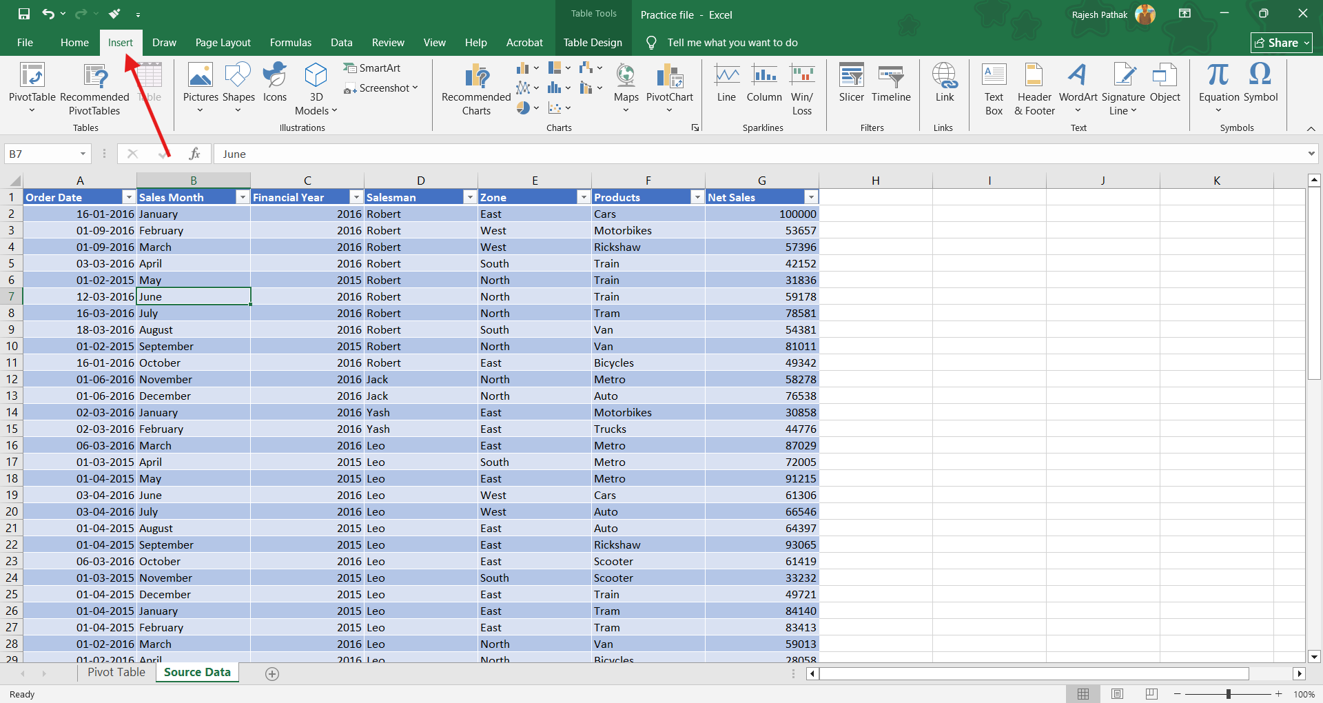
Go to insert ribbon tab.

Click on slicer 

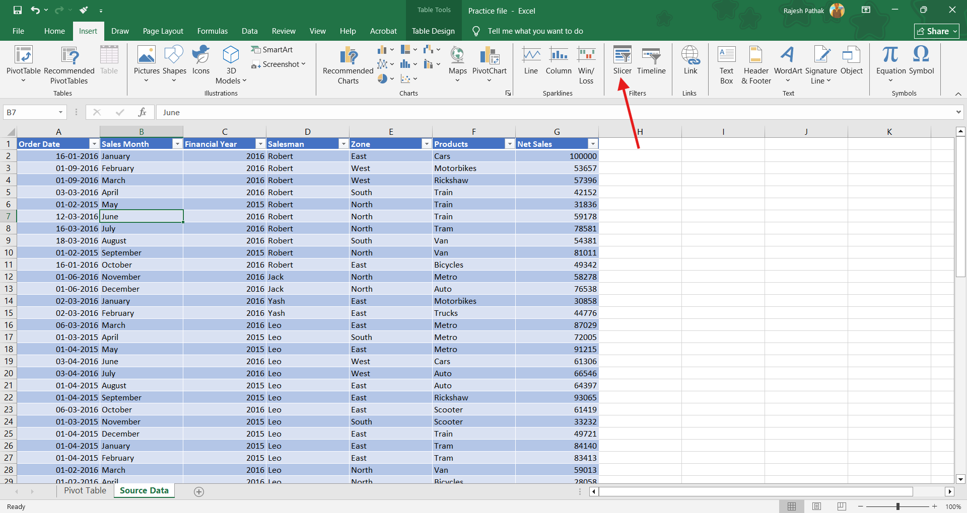
Select salesman. Press Ok.

Place the slicer in appropriate place. 

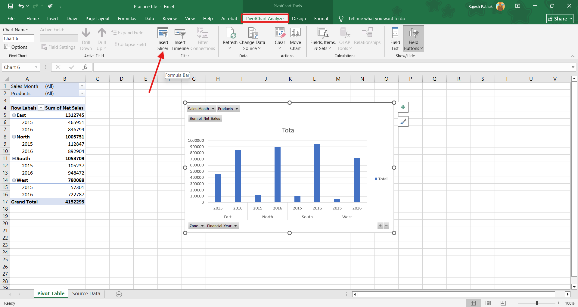
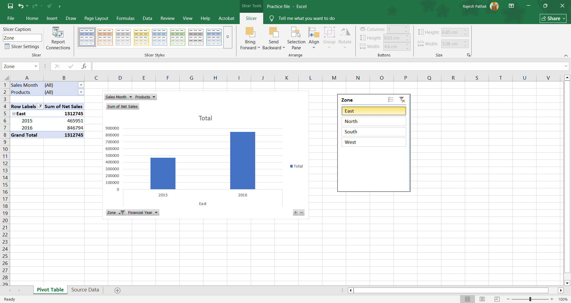
We can also use slicer in pivot chart.

Keep the pivot chart selected. From PivotChart Analyze ribbon tab, click on insert slicer.

Select Zone. Press Ok.

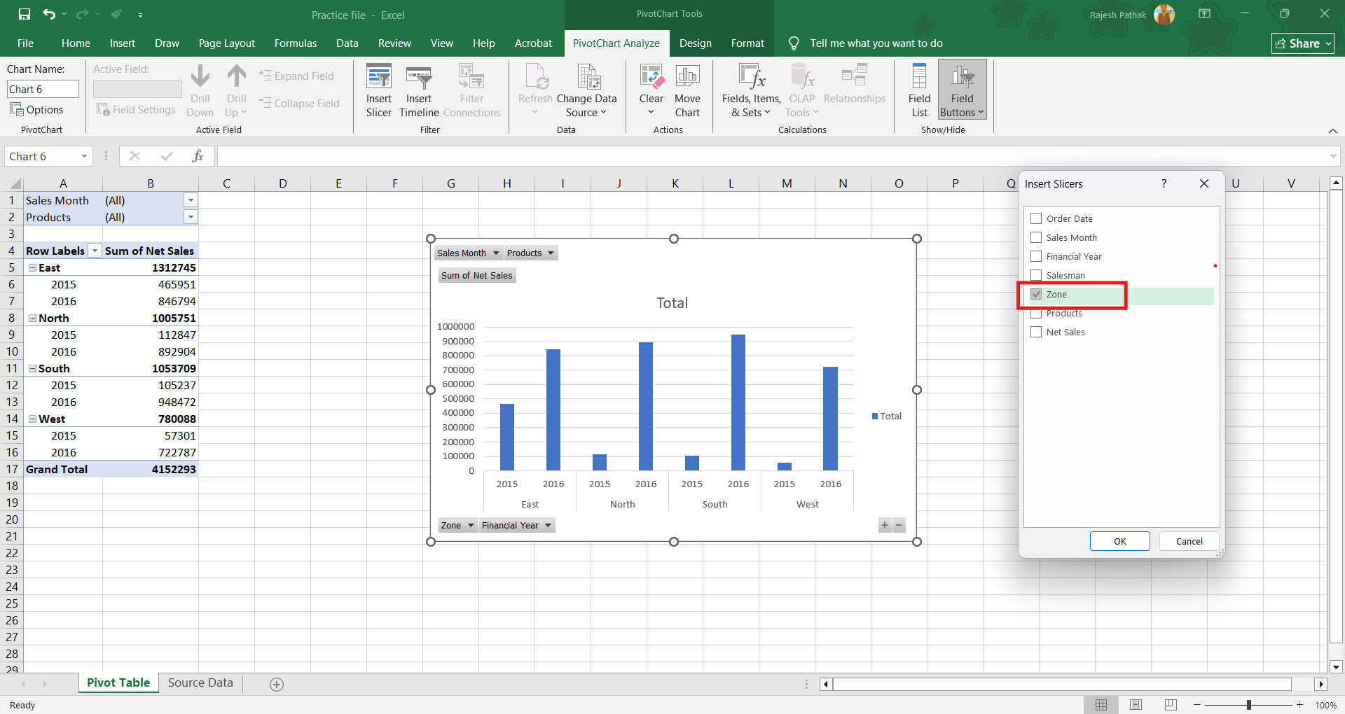
Clicking on slicer buttons change both pivot chart and pivot table.

When we click on slicer, it provides points for resizing it.

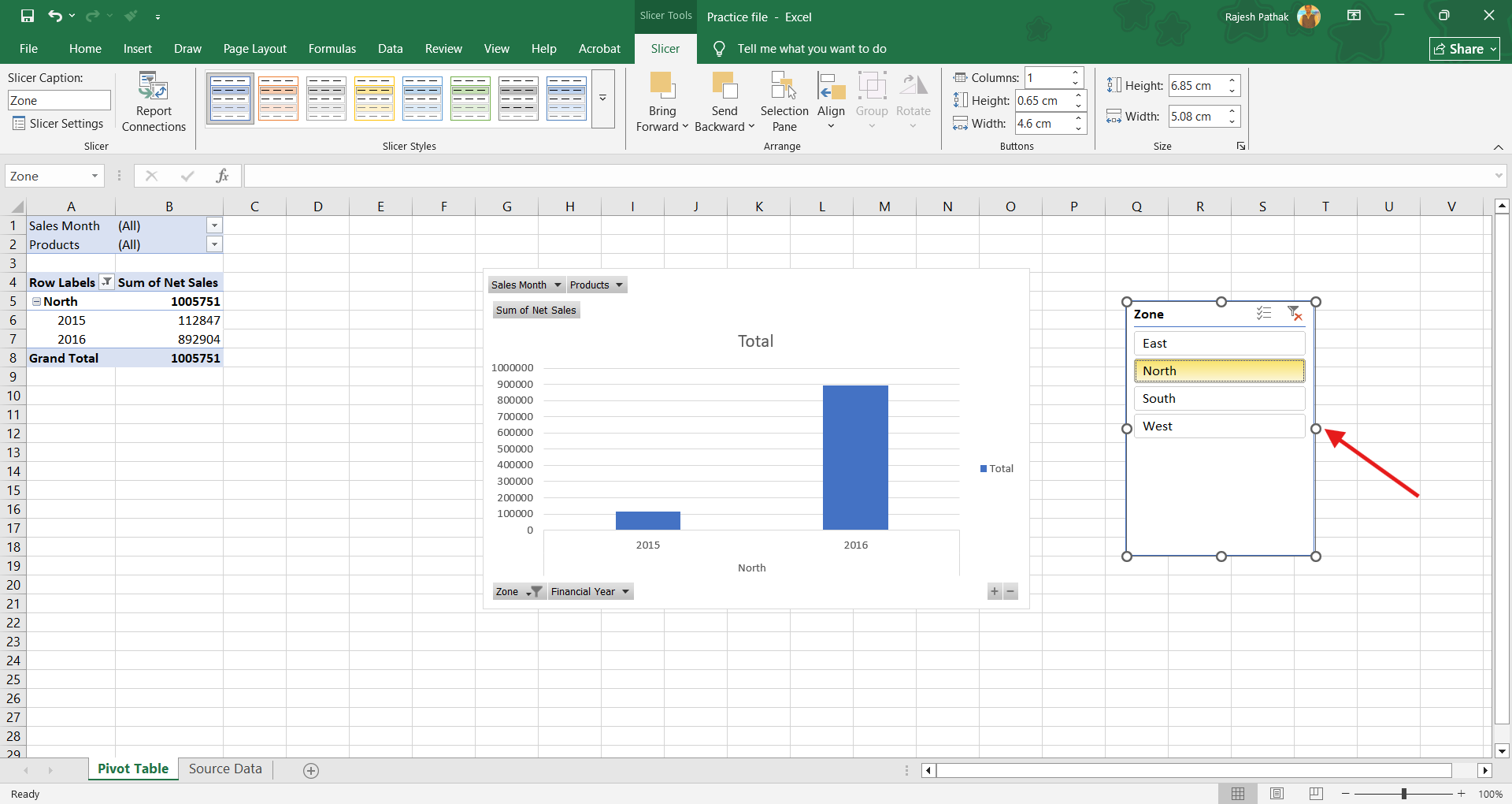
We can  move the slicer from its position by dragging. But we might not want others to change our slicer size and position when we share our workbooks.

Therefore, it is better to disable resizing and moving features of slicers.

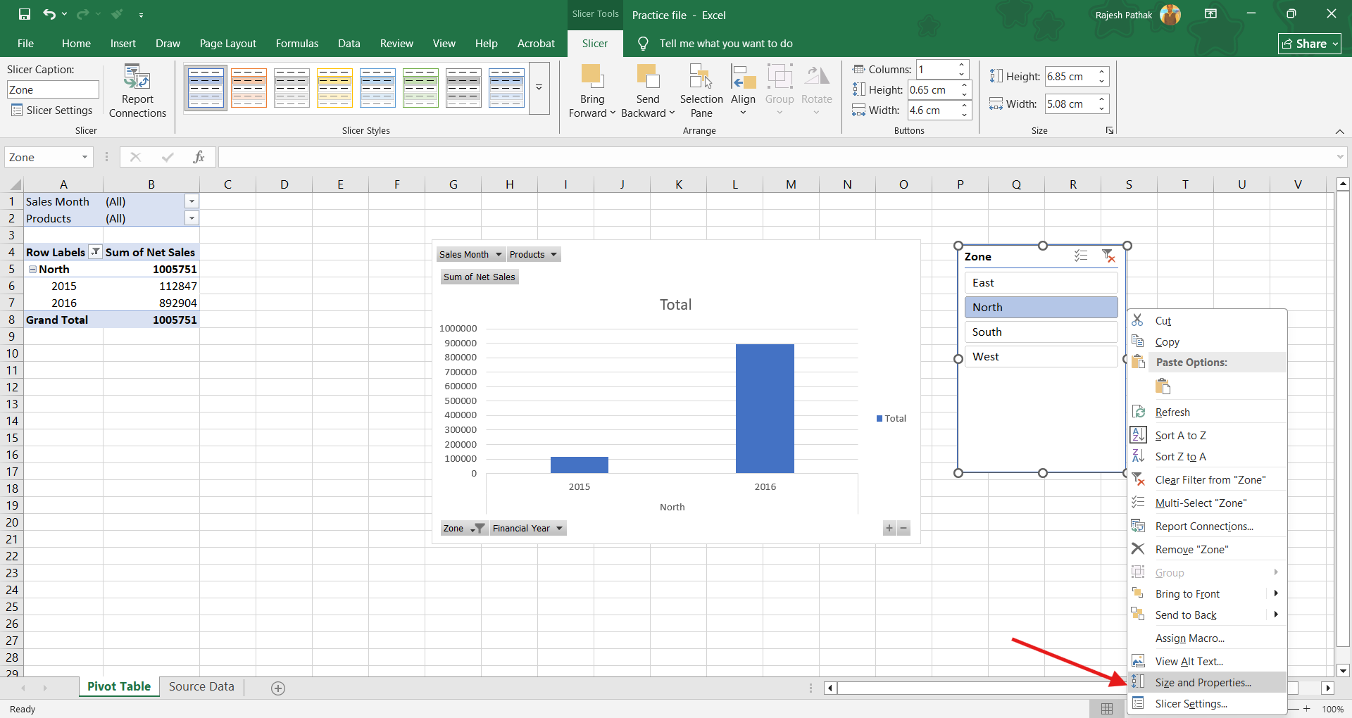
Right click on the slicer. Click on 'size and properties'.

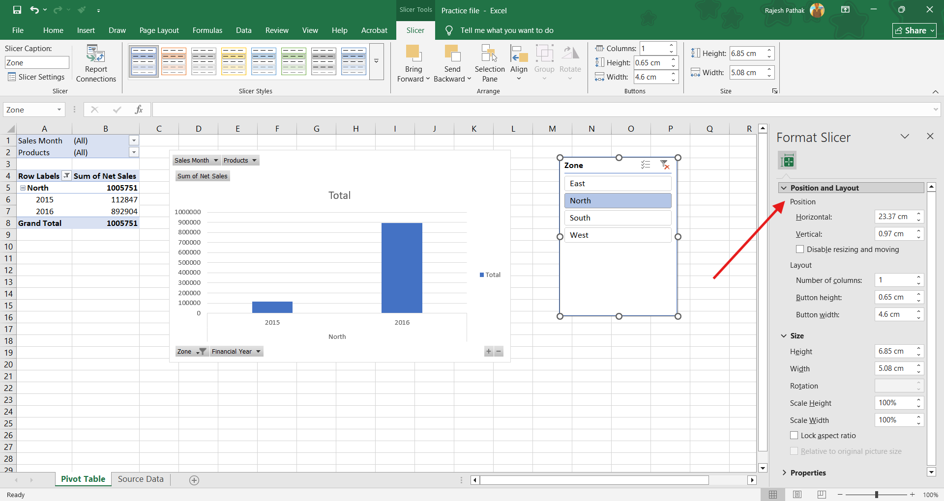
'Format slicer' window opens. Click on 'Position and Layout'.

Check 'disable resizing and moving' option.

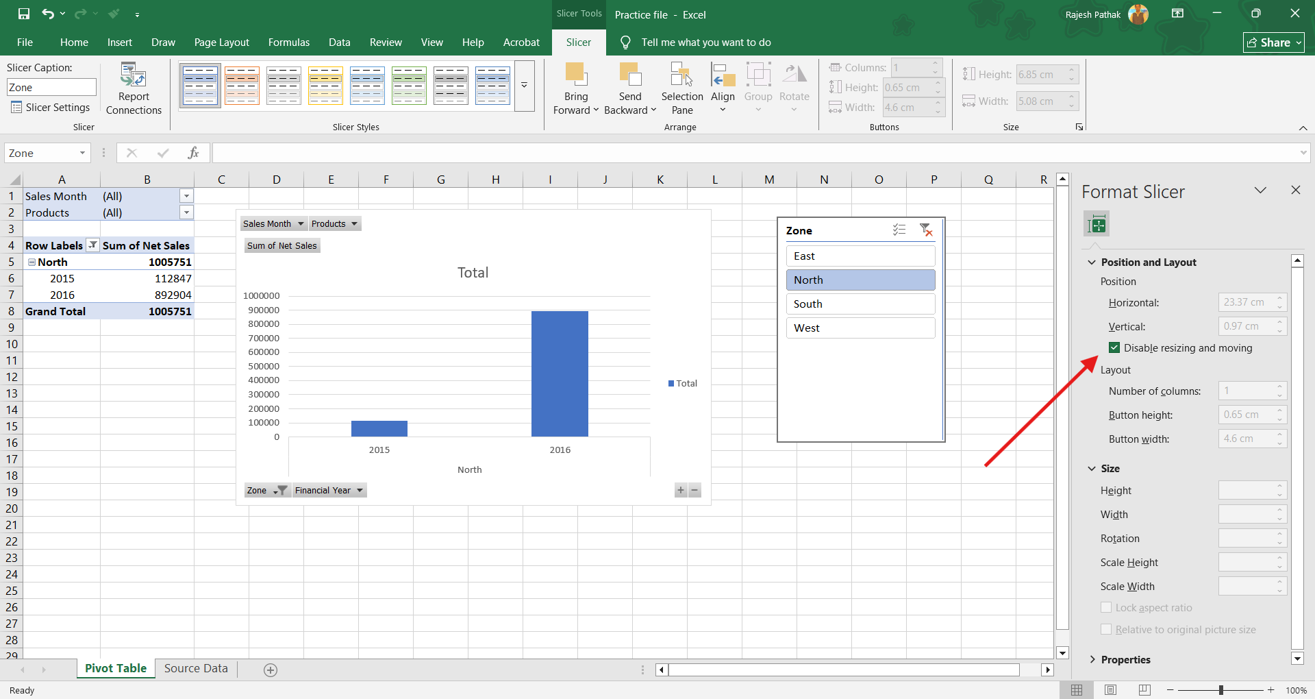
Close 'format slicer' window. Clicking on slicer buttons will still work. But no one can resize the slicer or move thc slicer.

Slicer can be cut from active worksheet......and pasted in another worksheet. Slicer will still filter the pivot table created in another worksheet.

If you found this post useful, you can say thanks in the comment section below. I would be happy to interact with you.  😊 

I’m a corporate trainer who teaches Microsoft Excel end‑to‑end: foundational spreadsheets and formulas, intermediate data tools, pivot tables, and analytics. Every program is hands‑on and role‑focused for individual learners or corporate cohorts. Click the link below to view course details, upcoming schedules and enrolment options.

MS Excel Data Management Programs